So, thanks to my former boss, and head of direct indexing at BNY Mellon, Vijay Vaidyanathan, and his Coursera course, along with the usual assistance from chatGPT (I officially see it as a pseudo programming language), I have some more software for the Python community now released to my github. As wordpress now makes it very difficult to paste formatted code, I’ll be linking more often to github files.
In today’s post, the code in question is a python file containing quite a few functions from R’s PerformanceAnalytics library outside of Return.portfolio (or Return_portfolio, as it may be in Python, because the . operator is reserved in Python…ugh).
Now, while a lot of the functions should be pretty straightforward (annualized return, VaR, CVaR, tracking error/annualized tracking error, etc.), two functions that I think are particularly interesting that I ported over from R with the help of chatGPT (seriously, when prompted correctly, an LLM is quite helpful in translating from one programming language to another, provided the programmer has enough background in both languages to do various debugging) are charts_PerformanceSummary, which does exactly what you might think it does from seeing me use the R function here on the blog, and table_Drawdowns, which gives the highest N drawdowns by depth.
Here’s a quick little Python demo (once you import my file from the github):
import yfinance as yf
import pandas as pd
import numpy as np

symbol = "SPY"
start_date = "1990-01-01"
end_date = pd.Timestamp.today().strftime("%Y-%m-%d")
df_list = []

data = pd.DataFrame(yf.download(symbol, start=start_date, end=end_date))
data = data["Adj Close"]
data.name = symbol
data = pd.DataFrame(data)

returns = Return_calculate(data)

charts_PerformanceSummary(returns)
table_Drawdowns(returns)
The NaT in the “To” column means that the drawdown is current, as does the NaN in the Recovery–they’re basically Python’s equivalent of NAs, though NaT means an NA on *time*, while an NaN means an NA on a numerical value. So that’s interesting in that Python gives you a little more information regarding your column data types, which is kind of interesting.
Another function included in this library, as a utility function is the infer_trading_periods function. Simply, plug in a time series, and it will tell you the periodicity of the data. Pandas was supposed to have a function that did this, but due to differences in frequency of daily data caused by weekends and holidays, this actually doesn’t work on financial data, so I worked with chatGPT to write a new function that works more generally. R’s checkData function is also in this library (translated over to Python), but I’m not quite sure where it was intended to be used, but left it in for those that want it.
So, for those interested, just feel free to read through some of the functions, and use whichever ones you find applicable to your workflow. That said, if you *do* wind up using it, please let me know, since there’s more value I can add.
So, it’s been a little while. But after a couple of years of some grunt work analytics jobs *and* consulting for a $1B AUM fund, I’ve decided that I had a bit more in the tank to share as far as quant content creation–quantent creation (?)–goes.
And a function I’ve searched for in Python for a long time now, but never finding it in a proper capacity is one that we’ve seen used time and again on this blog–R’s Return.portfolio.
For those uninitiated, Return.portfolio in R is essentially the workhorse of portfolio-level asset allocation backtests. What it does can be summarized in a sentence: given an xts/Python series dataframe of weights with m (E.G. 10) assets, and an xts/Python series dataframe with returns of m assets, Return.portfolio will compute drifted portfolio returns, along with beginning of period weights, end of period weights, beginning/end of period values, contribution to returns, and in the case of the Python variant that I wrote, two-way turnover.
Now, why is this function vital to have in Python, in my opinion?
Simple: because onto my experience with the language, if you want to do any financial research with Python, you need to learn some arcane and convoluted syntax such as zipline or quantconnect, and in some cases, that depends on working through another website altogether (in the case of quantconnect), or in the case of zipline, a library developed by a company that no longer exists (quantopian), so in either case, using either of these libraries may not be the best of ideas, even *if* you put in the who-knows-how-many-hours to learn a bunch of extra syntax fighting for real estate in your head.
Instead, what porting R’s Return.portfolio into Python does is to allow the same exact numpy/scipy/pandas ye-olde-classic-data-science syntax to not only work with backtesting, but also to seamlessly link up with whatever other Python library you may want to use, such as cvxpy for your portfolio optimization solutions (having used this library on past consulting arrangements, I am *very* impressed).
Now, here’s the link to my github for the code for Return.portfolio in Python–or, rather, since the dot operator has a special use in Python, the Return_portfolio function.
But for the record, here’s the Python code, including the endpoints function.
def endpoints(df, on = "M", offset = 0):
    """
    Returns index of endpoints of a time series analogous to R's endpoints
    function.
    Takes in:
        df -- a dataframe/series with a date index

        on -- a string specifying frequency of endpoints

        (E.G. "M" for months, "Q" for quarters, and so on)

        offset -- to offset by a specified index on the original data
        (E.G. if the data is daily resolution, offset of 1 offsets by a day)
        This is to allow for timing luck analysis. Thank Corey Hoffstein.
    """

    # to allow for familiarity with R
    # "months" becomes "M" for resampling
    if len(on) > 3:
        on = on[0].capitalize()

    # get index dates of formal endpoints
    ep_dates = pd.Series(df.index, index = df.index).resample(on).max()

    # get the integer indices of dates that are the endpoints
    date_idx = np.where(df.index.isin(ep_dates))

    # append last day to match R's endpoints function
    # remember, Python is indexed at 0, not 1
    #date_idx = np.insert(date_idx, 0, 0)
    date_idx = np.append(date_idx, df.shape[0]-1)
    if offset != 0:
        date_idx = date_idx + offset
        date_idx[date_idx < 0] = 0
        date_idx[date_idx > df.shape[0]-1] = df.shape[0]-1
    out = np.unique(date_idx)
    return out

def compute_weights_and_returns(subset_returns, weights):
  rep_weights = np.tile(weights, (len(subset_returns), 1))
  cum_subset_weights = np.cumprod(1 + subset_returns, axis=0) * rep_weights
  EOP_Weight = cum_subset_weights / np.sum(cum_subset_weights, axis=1).to_numpy()[:, np.newaxis]
  cum_subset_weights_bop = cum_subset_weights / (1 + subset_returns)
  BOP_Weight = cum_subset_weights_bop / np.sum(cum_subset_weights_bop, axis=1).to_numpy()[:, np.newaxis]
  portf_returns_subset = pd.DataFrame(np.sum(subset_returns.values * BOP_Weight, axis=1),
                                        index=subset_returns.index, columns=['Portfolio.Returns'])
  return [portf_returns_subset, BOP_Weight, EOP_Weight]


# Return.portfolio.geometric from R
def Return_portfolio(R, weights=None, verbose=True, rebalance_on='months'):
  """

    Parameters
    ----------
    R : a pandas series of asset returns
    weights : a vector or pandas series of asset weights.
    verbose : a boolean specifying a verbose output containing:
        portfolio returns,
        beginning of period weights and values, end of period weights and values,
        asset contribution to returns, and two-way turnover calculation
    rebalance_on : a string specifying rebalancing frequency if weights are passed in as a vector.

    Raises
    ------
    ValueError
        Number of asset weights must be equal to the number of assets.

    Returns
    -------
    TYPE
        See verbose parameter for True value, otherwise just portfolio returns.

    """

  # make sure original object isn't overridden
  R = R.copy()
  weights = weights.copy()

  # impute NAs in returns
  if R.isna().sum().sum() > 0:
    R.fillna(0, inplace=True)
    wn.warn("NAs detected in returns. Imputing with zeroes.")

    # if no weights provided, create equal weight vector
  if weights is None:
    weights = np.repeat(1/R.shape[1], R.shape[1])
    wn.warn("Weights not provided, assuming equal weight for rebalancing periods.")

    # if weights aren't passed in as a data frame (they're probably a list)
    # turn them into a 1 x num_assets data frame
  if type(weights) != pd.DataFrame:
    weights = pd.DataFrame(weights)
    weights = weights.transpose()

    # error checking for same number of weights as assets
  if weights.shape[1] != R.shape[1]:
        raise ValueError("Number of weights is unequal to number of assets. Correct this.")


  # if there's a row vector of weights, create a data frame with  the desired
  # rebalancing schedule --  also add in the very first date into the schedule
  if weights.shape[0] == 1:
        if rebalance_on is not None:
            ep = endpoints(R, on = rebalance_on)
            first_weights = pd.DataFrame(np.array(weights), index=[R.index[0]], columns=R.columns)
            weights = pd.concat([first_weights, pd.DataFrame(np.tile(weights,
                        (len(ep), 1)), index=R.index[ep], columns=R.columns)], axis=0)
            #weights = pd.DataFrame(np.tile(weights, (len(ep), 1)),
            #                       index = ep.index, columns = R.columns)
            weights.index.name = R.index.name
        else:
            weights = pd.DataFrame(weights, index=[R.index[0]], columns=R.columns)

  original_weight_dim = weights.shape[1] # save this for computing two-way turnover


  if weights.isna().sum().sum() > 0:
    weights.fillna(0, inplace=True)
    wn.warn("NAs detected in weights. Imputing with zeroes.")

  residual_weights = 1 - weights.sum(axis=1)
  if abs(residual_weights).sum() != 0:
    print("One or more periods do not have investment equal to 1. Creating residual weights.")
    weights["Residual"] = residual_weights
    R["Residual"] = 0

  if weights.shape[0] != 1:
    portf_returns, bop_weights, eop_weights = [], [], []
    for i in range(weights.shape[0]-1):
      subset = R.loc[(R.index >= weights.index[i]) & (R.index <= weights.index[i+1])]
      if i >= 1: # first period include all data
                # otherwise, final period of previous period is included, so drop it
        subset = subset.iloc[1:]
      subset_out = compute_weights_and_returns(subset, weights.iloc[i,:])
      subset_out[0].columns = ["Portfolio.Returns"]
      portf_returns.append(subset_out[0])
      bop_weights.append(subset_out[1])
      eop_weights.append(subset_out[2])
    portf_returns = pd.concat(portf_returns, axis=0)
    bop_weights = pd.concat(bop_weights, axis=0)
    eop_weights = pd.concat(eop_weights, axis=0)
  else: # only one weight allocation at the beginning and just drift the portfolio
    out = compute_weights_and_returns(R, weights)
    portf_returns = out[0]; portf_returns.columns = ['Portfolio.Returns']
    bop_weights = out[1]
    eop_weights = out[2]


  pct_contribution = R * bop_weights
  cum_returns = (1 + portf_returns).cumprod()
  eop_value = eop_weights * pd.DataFrame(np.tile(cum_returns, (1, eop_weights.shape[1])),
                                        index=eop_weights.index, columns=eop_weights.columns)
  bop_value = bop_weights * pd.DataFrame(np.tile(cum_returns/(1+portf_returns), (1, bop_weights.shape[1])),
                                        index=bop_weights.index, columns=bop_weights.columns)

  turnover = (np.abs(bop_weights.iloc[:, :(original_weight_dim-1)] - eop_weights.iloc[:, :(original_weight_dim-1)].shift(1))).sum(axis=1).dropna()
  turnover = pd.DataFrame(turnover, index=eop_weights.index[1:], columns=['Two-way turnover'])

  out = [portf_returns, pct_contribution, bop_weights, eop_weights, bop_value, eop_value, turnover]
  out = {k: v for k, v in zip(['returns', 'contribution', 'BOP.Weight', 'EOP.Weight', 'BOP.Value', 'EOP.Value', 'Two.Way.Turnover'], out)}
  if verbose:
        return out
  else:
        return portf_returns
Rather than go into it line by line, those interested can read the code, but ultimately, a lot of it is basically seeing if the weights were passed in as a data frame of individually customized weights (E.G. on January, my weights were such and such, and on February, they shifted to some other such and such), or if the weights were passed in as a vector, or Python list, if someone just wants to rebalance a portfolio (E.G. a classic buy-and-hold 60/40), and if some portfolio weights don’t add up to 1. Essentially, a fair bit of bookkeeping. (Speaking of, I’m not sure what happened to the programming language customization block here on wordpress, so, I sincerely encourage readers to check my github for this code).
Now, here’s the interesting part which motivated this post:
I didn’t write most of this code in Python. Or rather, not initially.
I wrote it in R, first, to understand it, with R’s vectorization, where I’m a bit more comfortable. (As an aside, as far as languages for quantitative finance go, I think R has the much more advanced buy-side libraries such as PortfolioAnalytics or Quantstrat compared to Python, as they were written by high-level industry practitioners, whereas Python’s finance ecosystem seems to be…fairly threadbare, consisting of various islands of libraries that don’t really play together all that well.)
Here’s the R code that I did to rewrite Peter Carl’s Return.portfolio.geometric (the underlying function that runs Return.portfolio that I’ve used all these years):
compute_weights_and_returns <- function(subset, weights) {
  rep_weights <- matrix(nrow=nrow(subset), ncol = ncol(subset), weights, byrow = TRUE)
  cum_subset_weights <- cumprod(1+subset) * rep_weights
  EOP.Weight <- cum_subset_weights/rowSums(cum_subset_weights)
  cum_subset_weights_bop <- cum_subset_weights/(1+subset)
  BOP.Weight <- cum_subset_weights_bop/rowSums(cum_subset_weights_bop)
  portf_returns_subset <- xts(rowSums(subset * BOP.Weight), order.by=index(subset))
  return(list(portf_returns_subset, BOP.Weight, EOP.Weight))
}

Return.portfolio.geometric.ilya <- function(R, weights, verbose = TRUE, rebalance_on = 'months') {

  if(sum(is.na(R)) > 0) {
    R[is.na(R)] <- 0
    warning("NAs detected in returns. Imputing with zeroes.")
  }

  if(missing(weights)) {
    weights <- rep(1/ncol(R), ncol(R))
    warning("Weights not provided, assuming equal weight for rebalancing periods.")
  }

  # if weights passed in as vector
  if(is.null(dim(weights))) {
    if(!is.null(rebalance_on)) {
      ep <- endpoints(R)
      first_weights <- xts(t(matrix(weights)), order.by=index(R)[1])
      weights <- rbind(first_weights,
                           xts(matrix(nrow=length(index(R)[ep]),
                                      ncol = length(weights), weights, byrow=TRUE),
                             order.by = index(R)[ep]))
      # get the first day of all the weights, make sure it's unique
      # weights <- weights[!duplicated(index(weights)),]
    } else {
      weights <- xts(t(matrix(weights)), order.by=index(R)[1])
    }
    colnames(weights) <- colnames(R)
  }

  original_weight_dim <- ncol(weights) # save this for computing two-way turnover

  if(original_weight_dim != ncol(R)) {
    stop("Number of weights is unequal to number of assets. Correct this.")
  }

  if(sum(is.na(weights)) > 0) {
    weights[is.na(weights)] <- 0
    warning("NAs detected in weights. Imputing with zeroes.")
  }

  residual_weights <- 1-rowSums(weights)
  if(sum(abs(residual_weights)) != 0) {
    warning("One or more periods do not have investment equal to 1. Creating residual weights.")
    weights$Residual <-  residual_weights
    R$Residual <- 0
  }
  if(nrow(weights) != 1) {
    portf_returns <- bop_weights <- eop_weights <- list()
    for(i in 1:(nrow(weights)-1)) {
      subset <- R[paste((index(weights)[i]),index(weights)[i+1], sep = "::"),]
      if(i >= 2) { # first period include all data
        # otherwise, final period of previous period is included, so drop it
        subset <- subset[-1,]
      }
      subset_out <- compute_weights_and_returns(subset, weights[i,])
      colnames(subset_out[[1]]) <- "Portfolio.Returns"
      portf_returns[[i]] <- subset_out[[1]]
      bop_weights[[i]] <- subset_out[[2]]
      eop_weights[[i]] <- subset_out[[3]]
    }
    portf_returns <- do.call(rbind, portf_returns)
    bop_weights <- do.call(rbind, bop_weights)
    eop_weights <- do.call(rbind, eop_weights)
  } else { # only one weight allocation at the beginning and just drift the portfolio
    out <- compute_weights_and_returns(R, weights)
    portf_returns <- out[[1]]; colnames(portf_returns) <- "Portfolio.Returns"
    bop_weights <- out[[2]]
    eop_weights <- out[[3]]
  }
  pct_contribution <- R * bop_weights
  cum_returns <- cumprod(1+portf_returns)
  eop_value <- eop_weights * matrix(nrow=nrow(eop_weights), ncol = ncol(eop_weights),
                                    cum_returns, byrow= FALSE)
  bop_value <- bop_weights * matrix(nrow=nrow(bop_weights), ncol = ncol(bop_weights),
                                    cum_returns/(1+portf_returns), byrow = FALSE)

  # add turnover computation because that's what this whole exercise is about
  turnover <- na.omit(xts(rowSums(abs(bop_weights[,1:original_weight_dim] -
                                        lag(eop_weights[,1:original_weight_dim]))),
                          order.by = index(eop_weights)))

  colnames(turnover) <- "Two-way turnover"

  out <- list(portf_returns, pct_contribution, bop_weights,
              eop_weights, bop_value, eop_value, turnover)
  names(out) <- c("returns", "contribution", "BOP.Weight",
                  "EOP.Weight", "BOP.Value", "EOP.Value", "Two.Way.Turnover")
  if(verbose) {
    return(out)
  } else {
    return(portf_returns)
  }
}
Now, how did I go from the above to the code at the beginning of this post?
ChatGPT4.
That is, I translated my R code into Python code using ChatGPT4 by simply having it translate, block by block, my R code into Python.
Now, was it perfect? No, actually. I had to run the code block by block, and do a little bit of debugging here and there–including adding the functionality for the Return_portfolio function to make deep copies of the returns and weights, instead of modifying the original data structure passed into the function, since Python by default is a pass by reference language, not pass by value (ugh). However, this sort of “Rosetta Stone” functionality inherent in ChatGPT4 is occasionally useful.
Now, when I first tried prompting chatGPT4 to just translate R’s functions, without guiding it step by step, it was a total disaster. Contrary to popular belief, ChatGPT4 is *not* some all-powerful, all-perfect, all-knowing, and all-wise (as the late, great, George Carlin once said) system. But occasionally, it can be useful.
Furthermore, as someone that’s used AI to try my hand at image generation, I also consider those systems (such as StableDiffusion, or Leonardo.AI) to be…somewhat impressive, if in their infancy right now (it gets much more difficult to have multiple subjects interact on one image–I.E. if you want to describe one person in an image, that’s one thing, but if you want to describe two, it isn’t like you can make an image of one–say, save it with a name, such as Alice.jpeg, make an image of a second, save it to another name, such as Bob.jpeg, and then say “Alice being hugged by Bob”). Of course, I’ve definitely been aware about the copyright hubbub brewing over the image generating AI space, but as someone that’s given away plenty of code over the past 8 or so years, including code that has been augmented to run $87 million at a $1B AUM fund, I’m pretty squarely on the open source side, even if seeing my code being responsible for running more than $100 million in AUM, and not getting paid residuals on the management fees, has discouraged me from continuing to share strategy research (I was always of the opinion that anything I shared using freely available Yahoo data was something that large investment houses had already passed over and run a more sophisticated variant of–apparently, this isn’t the case, so giving away strategy code for free nowadays seems like a very suspect thing to do).
In any case, using image-generating AI has allowed me to make artwork the likes of which I never dreamed of creating before, so I’m of the opinion that a few people taking the side of IP hoarding corporations (such as big pharma hoarding insulin patents, or Disney continuing to milk Mickey Mouse) can go kick rocks, and that IP law has long overreached. That said, I already have StableDiffusion running on my machine, coupled with some more sophisticated models built on top of it (Dreamshaper v5, Deliberate v2, etc.), and still have a lot to learn about it–though I’ll probably need a more powerful machine than a gaming laptop to really crank images out.
Now, my thoughts on AI? So far, I don’t think that AI alone is going to pull a South Park and DERK YERRR JERBZ. At least if you’re a skilled professional.
Not alone, anyway. And for what it’s worth, as a quantitative research analyst, I found that I’d fire ChatGPT4 within a few hours, owing to the artifact of AI hallucinations. As the phrase goes, trust *but verify*. I think we’re still far, far away from ChatGPT4 being able to read a strategy paper on Quantpedia, replicating it in R or Python, running the code, and replicating the results. For that matter, I think that any strategy paper submission or blog post is incomplete without data and code, for immediate replication, ready to go. It’s the 21st century. Github or git out. A minimum reproducible example (MRE) as a demo of the concept (even a toy one), in my opinion, is vastly more useful than 25 pages of mathematical derivation. Though that’s just me speaking given my background of hands-on engineering and actually *doing things* rather than merely theorizing about them.
Okay, so…this post seems to have gotten long in the tooth. In other news, I’m in the job market, currently, and as I’ve shown, I have a fairly solid command of Python, having several years of off and on experience with it. And I’m also wondering if a written blog is the best way to actually communicate so many of my findings, or if YouTube is the way to go (though I don’t know much about editing videos).
So…yeah. Follow if you like the post, and most importantly:
First off, for the hiring managers out there, after about a one-year contracting role at Bank of America doing some analytical reporting coding for them in Python, I am on the job market. Feel free to find my LinkedIn here.
This post will cover how to make tactical asset allocation strategies a bit more realistic with regards to execution. That is, by using next-day open-to-open rather than observe-the-close-get-the-close, it’s possible to see how much this change affects a strategy, and potentially, something that I think a site like AllocateSmartly could implement to actively display in their simulations (E.G. a checkbox that says “display next-day open to open returns”).
Now, onto the idea of the post: generally, when doing tactical asset allocation backtests, we tend to just use one set of daily returns. Get the adjusted close data, and at the end of every month, allocate to selected holdings. That is, most TAA backtests we’ve seen generally operate under the assumption of:
“Run the program at 3:50 PM EST. on the last day of the month, scrape the prices for the assets, allocate assets in the next ten minutes.”
This…can generally work for small accounts, but for institutions interested in scaling these strategies, maybe not so much.
So, the trick here, first, in English is this:
Compute open-to-open returns. Lag them by negative one. While this may sound really spooky at first, because a lag of negative one implies the potential for lookahead bias, in this case, it’s carefully done to use future returns. That is, the statement in English is (for example): “given my weights for data at the close of June 30, what would my open-to-open returns have been if I entered on the open of July 1st, instead of the June 30 close?”. Of course, this sets the return dates off by one day, so you’ll have to lag the total portfolio returns by a positive one to readjust for that.
require(quadprog)

# compute strategy statistics
stratStats <- function(rets) {
  stats <- rbind(table.AnnualizedReturns(rets), maxDrawdown(rets))
  stats[5,] <- stats[1,]/stats[4,]
  stats[6,] <- stats[1,]/UlcerIndex(rets)
  rownames(stats)[4] <- "Worst Drawdown"
  rownames(stats)[5] <- "Calmar Ratio"
  rownames(stats)[6] <- "Ulcer Performance Index"
  return(stats)
}

# required libraries
require(quantmod)
require(PerformanceAnalytics)
require(tseries)

# symbols
symbols <- c("SPY", "VGK",   "EWJ",  "EEM",  "VNQ",
"RWX",  "IEF",  "TLT",  "DBC",  "GLD", "VWO", "BND")


# get data
rets <- list()
prices <- list()
op_rets <- list()
for(i in 1:length(symbols)) {
  tmp <- getSymbols(symbols[i], from = '1990-01-01', auto.assign = FALSE, use.adjusted = TRUE)
  price <- Ad(tmp)
  returns <- Return.calculate(Ad(tmp))
  op_ret <- Return.calculate(Op(tmp))
  colnames(returns) <- colnames(price) <- colnames(op_ret) <- symbols[i]
  prices[[i]] <- price
  rets[[i]] <- returns
  op_rets[[i]] <- op_ret
}
rets <- na.omit(do.call(cbind, rets))
prices <- na.omit(do.call(cbind, prices))
op_rets <- na.omit(do.call(cbind, op_rets))

# algorithm
KDA <- function(rets, offset = 0, leverageFactor = 1, momWeights = c(12, 4, 2, 1),
                op_rets = NULL, use_op_rets = FALSE) {

  # get monthly endpoints, allow for offsetting ala AllocateSmartly/Newfound Research
  ep <- endpoints(rets) + offset
  ep[ep < 1] <- 1
  ep[ep > nrow(rets)] <- nrow(rets)
  ep <- unique(ep)
  epDiff <- diff(ep)
  if(last(epDiff)==1) { # if the last period only has one observation, remove it
    ep <- ep[-length(ep)]
  }

  # initialize vector holding zeroes for assets
  emptyVec <- data.frame(t(rep(0, 10)))
  colnames(emptyVec) <- symbols[1:10]


  allWts <- list()
  # we will use the 13612F filter
  for(i in 1:(length(ep)-12)) {

    # 12 assets for returns -- 2 of which are our crash protection assets
    retSubset <- rets[c((ep[i]+1):ep[(i+12)]),]
    epSub <- ep[i:(i+12)]
    sixMonths <- rets[(epSub[7]+1):epSub[13],]
    threeMonths <- rets[(epSub[10]+1):epSub[13],]
    oneMonth <- rets[(epSub[12]+1):epSub[13],]

    # computer 13612 fast momentum
    moms <- Return.cumulative(oneMonth) * momWeights[1] + Return.cumulative(threeMonths) * momWeights[2] +
      Return.cumulative(sixMonths) * momWeights[3] + Return.cumulative(retSubset) * momWeights[4]
    assetMoms <- moms[,1:10] # Adaptive Asset Allocation investable universe
    cpMoms <- moms[,11:12] # VWO and BND from Defensive Asset Allocation

    # find qualifying assets
    highRankAssets <- rank(assetMoms) >= 6 # top 5 assets
    posReturnAssets <- assetMoms > 0 # positive momentum assets
    selectedAssets <- highRankAssets & posReturnAssets # intersection of the above

    # perform mean-variance/quadratic optimization
    investedAssets <- emptyVec
    if(sum(selectedAssets)==0) {
      investedAssets <- emptyVec
    } else if(sum(selectedAssets)==1) {
      investedAssets <- emptyVec + selectedAssets
    } else {
      idx <- which(selectedAssets)
      # use 1-3-6-12 fast correlation average to match with momentum filter
      cors <- (cor(oneMonth[,idx]) * momWeights[1] + cor(threeMonths[,idx]) * momWeights[2] +
                 cor(sixMonths[,idx]) * momWeights[3] + cor(retSubset[,idx]) * momWeights[4])/sum(momWeights)
      vols <- StdDev(oneMonth[,idx]) # use last month of data for volatility computation from AAA
      covs <- t(vols) %*% vols * cors

      # do standard min vol optimization
      minVolRets <- t(matrix(rep(1, sum(selectedAssets))))

      n.col = ncol(covs)
      zero.mat <- array(0, dim = c(n.col, 1))
      one.zero.diagonal.a <- cbind(1, diag(n.col), 1 * diag(n.col), -1 * diag(n.col))
      min.wgt <- rep(.05, n.col)
      max.wgt <- rep(1, n.col)
      bvec.1.vector.a <- c(1, rep(0, n.col), min.wgt, -max.wgt)
      meq.1 <- 1

      mv.port.noshort.a <- solve.QP(Dmat = covs, dvec = zero.mat, Amat = one.zero.diagonal.a,
                                    bvec = bvec.1.vector.a, meq = meq.1)

      min_vol_wt <- mv.port.noshort.a$solution
      names(min_vol_wt) <- rownames(covs)

      #minVolWt <- portfolio.optim(x=minVolRets, covmat = covs)$pw
      #names(minVolWt) <- colnames(covs)
      investedAssets <- emptyVec
      investedAssets[,selectedAssets] <- min_vol_wt
    }

    # crash protection -- between aggressive allocation and crash protection allocation
    pctAggressive <- mean(cpMoms > 0)
    investedAssets <- investedAssets * pctAggressive

    pctCp <- 1-pctAggressive

    # if IEF momentum is positive, invest all crash protection allocation into it
    # otherwise stay in cash for crash allocation
    if(assetMoms["IEF"] > 0) {
      investedAssets["IEF"] <- investedAssets["IEF"] + pctCp
    }

    # leverage portfolio if desired in cases when both risk indicator assets have positive momentum
    if(pctAggressive == 1) {
      investedAssets = investedAssets * leverageFactor
    }

    # append to list of monthly allocations
    wts <- xts(investedAssets, order.by=last(index(retSubset)))
    allWts[[i]] <- wts

  }

  # put all weights together and compute cash allocation
  allWts <- do.call(rbind, allWts)
  allWts$CASH <- 1-rowSums(allWts)

  # add cash returns to universe of investments
  investedRets <- rets[,1:10]

  investedRets$CASH <- 0

  # compute portfolio returns
  out <- Return.portfolio(R = investedRets, weights = allWts)
  if(use_op_rets) {
    if(is.null(op_rets)) {
      stop("You didn't provide open returns.")
    } else {
      # cbind a cash return of 0 -- may not be necessary in current iterations of PerfA
      investedRets <- cbind(lag(op_rets[,1:10], -1), 0)
      out <- lag(Return.portfolio(R = investedRets, weights = allWts))
    }
  }
  return(list(allWts, out))
}
Essentially, the salient part of the code is at the start, around line 32, when the algorithm gets the data from Yahoo, in that it creates a new set of returns using open adjusted data, and at the end, at around line 152, when the code lags the open returns by -1–I.E. lag(op_rets[,1:10], -1), and then lags the returns again to realign the correct dates–out <- lag(Return.portfolio(R=investedRets, weights = allWts))
As one can see, there’s definitely a bit of a performance deterioration to the tune of about 2% per year. While the strategy may still be solid, a loss of 20% of the CAGR means that the other risk/reward statistics suffer proportionally as well. In other words, this is a strategy that is fairly sensitive to the exact execution due to its fairly high turnover.
However, the good news is that there is a way to considerably reduce turnover as suggested by AllocateSmartly, which would be to reduce the impact of relative momentum on turnover. A new post on how to do *that* will be forthcoming in the near future.
One last thing–as I did pick up some Python skills, as evidenced by the way I ported the endpoints function into Python, and the fact that I completed an entire Python data science bootcamp in four instead of six months, I am also trying to port over the Return.portfolio function into Python as well, since that would allow a good way to compute turnover statistics as well. However, as far as I’ve seen with Python, I’m not sure there’s a well-maintained library similar to PerformanceAnalytics, and I do not know that there are libraries in Python that compare with rugarch, PortfolioAnalytics, and Quantstrat, though if anyone wants to share the go-to generally-accepted Python libraries to use beyond the usual numpy/pandas/matplotlib/cvxpy/sklearn (AKA the usual data science stack).
Thanks for reading.
NOTE: Lastly, some other news: late last year, I was contacted by the NinjaTrader folks to potentially become a vendor/give lectures on the NinjaTrader site about how to create quantitative/systematic strategies. While I’m not a C# coder, I can potentially give lectures on how to use R (and maybe Python in the future) to implement them.
Finally, if you wish to get in touch with me, my email is ilya.kipnis@gmail.com, and I can be found on my LinkedIn. Additionally, if you wish to subscribe to my volatility strategy, that I’ve been successfully trading since 2017, feel free to check it out here.
This post will detail a rather important finding I found while implementing a generalized framework for momentum asset allocation backtests. Namely, that when computing momentum (and other financial measures for use in asset allocation, such as volatility and correlations), measuring formal months, from start to end, has a large effect on strategy performance.
So, first off, I am in the job market, and am actively looking for a full-time role (preferably in New York City, or remotely), or a long-term contract. Here is my resume, and here is my LinkedIn profile. Furthermore, I’ve been iterating on my volatility strategy, and given that I’ve seen other services with large drawdowns, or less favorable risk/reward profiles charge $50/month, I think following my trades can be a reasonable portfolio diversification tool. Read about it and subscribe here. I believe that my body of work on this blog speaks to the viability of employing me, though I am also learning Python to try and port over my R skills over there, as everyone seems to want Python, and R much less so, hence the difficulty transferring between opportunities.
Anyhow, one thing I am working on is a generalized framework for tactical asset allocation (TAA) backtests. Namely, those that take the form of “sort universe by momentum, apply diversification weighting scheme”–namely, the kinds of strategies that the folks over at AllocateSmartly deal in. I am also working on this framework and am happy to announce that as of the time of this writing, I will happily work with individuals that want more customized TAA backtests, as the AllocateSmartly FAQs state that AllocateSmartly themselves do not do custom backtests. The framework I am currently in the process of implementing is designed to do just that. However, after going through some painstaking efforts to compare apples to apples, I came across a very important artifact. Namely, that there is a fairly large gulf in performance between measuring months from their formal endpoints, as opposed to simply approximating months with 21-day chunks (E.G. 21 days for 1 month, 63 for 3, and so on).
Here’s the code I’ve been developing recently–the long story short, is that the default options essentially default to Adaptive Asset Allocation, but depending on the parameters one inputs, it’s possible to get to something as simple as dual momentum (3 assets, invest in top 1), or as complex as KDA, with options to fine-tune it even further, such as to account for the luck-based timing that Corey Hoffstein at Newfound Research loves to write about (speaking of whom, he and the awesome folks at ReSolve Asset Management have launched a new ETF called ROMO–Robust Momentum–I recently bought a bunch in my IRA because a buy-it-and-forget-it TAA ETF is pretty fantastic as far as buy-and-hold investments go). Again, I set a bunch of defaults in the parameters so that most of them can be ignored.
require(PerformanceAnalytics)
require(quantmod)
require(tseries)
require(quadprog)

stratStats <- function(rets) {
  stats <- rbind(table.AnnualizedReturns(rets), maxDrawdown(rets))
  stats[5,] <- stats[1,]/stats[4,]
  stats[6,] <- stats[1,]/UlcerIndex(rets)
  rownames(stats)[4] <- "Worst Drawdown"
  rownames(stats)[5] <- "Calmar Ratio"
  rownames(stats)[6] <- "Ulcer Performance Index"
  return(stats)
}


getYahooReturns <- function(symbols, return_column = "Ad") {
  returns <- list()
  for(symbol in symbols) {
    getSymbols(symbol, from = '1990-01-01', adjustOHLC = TRUE)
    if(return_column == "Ad") {
      return <- Return.calculate(Ad(get(symbol)))
      colnames(return) <- gsub("\\.Adjusted", "", colnames(return))
    } else {
      return <- Return.calculate(Op(get(symbol)))
      colnames(return) <- gsub("\\.Open", "", colnames(return))

    }
    returns[[symbol]] <- return
  }
  returns <- na.omit(do.call(cbind, returns))
  return(returns)
}

symbols <- c("SPY", "VGK",   "EWJ",  "EEM",  "VNQ",  "RWX",  "IEF",  "TLT",  "DBC",  "GLD")

returns <- getYahooReturns(symbols)
canary <- getYahooReturns(c("VWO", "BND"))

# offsets endpoints by a certain amount of days (I.E. 1-21)
dailyOffset <- function(ep, offset = 0) {

  ep <- ep + offset
  ep[ep < 1] <- 1
  ep[ep > nrow(returns)] <- nrow(returns)
  ep <- unique(ep)
  epDiff <- diff(ep)
  if(last(epDiff)==1) {
    # if the last period only has one observation, remove it
    ep <- ep[-length(ep)]
  }
  return(ep)
}

# computes total weighted momentum and penalizes new assets (if desired)
compute_total_momentum <- function(yearly_subset,
                                   momentum_lookbacks, momentum_weights,
                                   old_weights, new_asset_mom_penalty) {

  empty_vec <- data.frame(t(rep(0, ncol(yearly_subset))))
  colnames(empty_vec) <- colnames(yearly_subset)

  total_momentum <- empty_vec
  for(j in 1:length(momentum_lookbacks)) {
    momentum_subset <- tail(yearly_subset, momentum_lookbacks[j])
    total_momentum <- total_momentum + Return.cumulative(momentum_subset) *
      momentum_weights[j]
  }

  # if asset returns are negative, penalize by *increasing* negative momentum
  # this algorithm assumes we go long only
  total_momentum[old_weights == 0] <- total_momentum[old_weights==0] *
    (1-new_asset_mom_penalty * sign(total_momentum[old_weights==0]))

  return(total_momentum)
}

# compute weighted correlation matrix
compute_total_correlation <- function(data, cor_lookbacks, cor_weights) {

  # compute total correlation matrix
  total_cor <- matrix(nrow=ncol(data), ncol=ncol(data), 0)
  rownames(total_cor) <- colnames(total_cor) <- colnames(data)
  for(j in 1:length(cor_lookbacks)) {
    total_cor = total_cor + cor(tail(data, cor_lookbacks[j])) * cor_weights[j]
  }

  return(total_cor)
}

# computes total weighted volatility
compute_total_volatility <- function(data, vol_lookbacks, vol_weights) {
  empty_vec <- data.frame(t(rep(0, ncol(data))))
  colnames(empty_vec) <- colnames(data)

  # normalize weights if not already normalized
  if(sum(vol_weights) != 1) {
    vol_weights <- vol_weights/sum(vol_weights)
  }

  # compute total volrelation matrix
  total_vol <- empty_vec
  for(j in 1:length(vol_lookbacks)) {
    total_vol = total_vol + StdDev.annualized(tail(data, vol_lookbacks[j])) * vol_weights[j]
  }

  return(total_vol)
}

check_valid_parameters <- function(mom_lookbacks, cor_lookbacks, mom_weights, cor_weights, vol_weights, vol_lookbacks) {
  if(length(mom_weights) != length(mom_lookbacks)) {
    stop("Momentum weight length must be equal to momentum lookback length.") }

  if(length(cor_weights) != length(cor_lookbacks)) {
    stop("Correlation weight length must be equal to correlation lookback length.")
  }

  if(length(vol_weights) != length(vol_lookbacks)) {
    stop("Volatility weight length must be equal to volatility lookback length.")
  }
}


# computes weights as a function proportional to the inverse of total variance
invVar <- function(returns, lookbacks, lookback_weights) {
  var <- compute_total_volatility(returns, lookbacks, lookback_weights)^2
  invVar <- 1/var
  return(invVar/sum(invVar))
}

# computes weights as a function proportional to the inverse of total volatility
invVol <- function(returns, lookbacks, lookback_weights) {
  vol <- compute_total_volatility(returns, lookbacks, lookback_weights)
  invVol <- 1/vol
  return(invVol/sum(invVol))
}

# computes equal weight portfolio
ew <- function(returns) {
  return(StdDev(returns)/(StdDev(returns)*ncol(returns)))
}

# computes minimum volatility portfolio
minVol <- function(returns, cor_lookbacks, cor_weights, vol_lookbacks, vol_weights) {
  vols <- compute_total_volatility(returns, vol_lookbacks, vol_weights)
  cors <- compute_total_correlation(returns, cor_lookbacks, cor_weights)
  covs <- t(vols) %*% as.numeric(vols) * cors
  min_vol_rets <- t(matrix(rep(1, ncol(covs))))

  n.col = ncol(covs)
  zero.mat <- array(0, dim = c(n.col, 1))
  one.zero.diagonal.a <- cbind(1, diag(n.col), 1 * diag(n.col), -1 * diag(n.col))
  min.wgt <- rep(0, n.col)
  max.wgt <- rep(1, n.col)
  bvec.1.vector.a <- c(1, rep(0, n.col), min.wgt, -max.wgt)
  meq.1 <- 1

  mv.port.noshort.a <- solve.QP(Dmat = covs, dvec = zero.mat, Amat = one.zero.diagonal.a,
                                bvec = bvec.1.vector.a, meq = meq.1)


  min_vol_wt <- mv.port.noshort.a$solution
  names(min_vol_wt) <- rownames(covs)
  return(min_vol_wt)
}
asset_allocator <- function(returns,
                           canary_returns = NULL, # canary assets for KDA algorithm and similar

                           mom_threshold = 0, # threshold momentum must exceed
                           mom_lookbacks = 126, # momentum lookbacks for custom weights (EG 1-3-6-12)

                           # weights on various momentum lookbacks (EG 12/19, 4/19, 2/19, 1/19)
                           mom_weights = rep(1/length(mom_lookbacks),
                                             length(mom_lookbacks)),

                           # repeat for correlation weights
                           cor_lookbacks = mom_lookbacks, # correlation lookback
                           cor_weights = rep(1/length(mom_lookbacks),
                                             length(mom_lookbacks)),

                           vol_lookbacks = 20, # volatility lookback
                           vol_weights = rep(1/length(vol_lookbacks),
                                             length(vol_lookbacks)),

                           # number of assets to hold (if all above threshold)
                           top_n = floor(ncol(returns)/2),

                           # diversification weight scheme (ew, invVol, invVar, minVol, etc.)
                           weight_scheme = "minVol",

                           # how often holdings rebalance
                           rebalance_on = "months",

                           # how many days to offset rebalance period from end of month/quarter/year
                           offset = 0,

                           # penalize new asset mom to reduce turnover
                           new_asset_mom_penalty = 0,

                           # run Return.Portfolio, or just return weights?
                           # for use in robust momentum type portfolios
                           compute_portfolio_returns = TRUE,
                           verbose = FALSE,

                           # crash protection asset
                           crash_asset = NULL,
                           ...
                           ) {

  # normalize weights
  mom_weights <- mom_weights/sum(mom_weights)
  cor_weights <- cor_weights/sum(cor_weights)
  vol_weights <- vol_weights/sum(vol_weights)

  # if we have canary returns (I.E. KDA strat), align both time periods
  if(!is.null(canary_returns)) {
   smush <- na.omit(cbind(returns, canary_returns))
   returns <- smush[,1:ncol(returns)]
   canary_returns <- smush[,-c(1:ncol(returns))]
   empty_canary_vec <- data.frame(t(rep(0, ncol(canary_returns))))
   colnames(empty_canary_vec) <- colnames(canary_returns)
  }

  # get endpoints and offset them
  ep <- endpoints(returns, on = rebalance_on)
  ep <- dailyOffset(ep, offset = offset)

  # initialize vector holding zeroes for assets
  empty_vec <- data.frame(t(rep(0, ncol(returns))))
  colnames(empty_vec) <- colnames(returns)
  weights <- empty_vec

  # initialize list to hold all our weights
  all_weights <- list()

  # get number of periods per year
  switch(rebalance_on,
         "months" = { yearly_periods = 12},
         "quarters" = { yearly_periods = 4},
         "years" = { yearly_periods = 1})

  for(i in 1:(length(ep) - yearly_periods)) {

    # remember old weights for the purposes of penalizing momentum of new assets
    old_weights <- weights

    # subset one year of returns, leave off first day
    return_subset <- returns[c((ep[i]+1):ep[(i+yearly_periods)]),]

    # compute total weighted momentum, penalize potential new assets if desired
    momentums <- compute_total_momentum(return_subset,
                                        momentum_lookbacks = mom_lookbacks,
                                        momentum_weights = mom_weights,
                                        old_weights = old_weights,
                                        new_asset_mom_penalty = new_asset_mom_penalty)

    # rank negative momentum so that best asset is ranked 1 and so on
    momentum_ranks <- rank(-momentums)
    selected_assets <- momentum_ranks <= top_n & momentums > mom_threshold
    selected_subset <- return_subset[, selected_assets]

    # case of 0 valid assets
    if(sum(selected_assets)==0) {
      weights <- empty_vec
    } else if (sum(selected_assets)==1) {

      # case of only 1 valid asset -- invest everything into it
      weights <- empty_vec + selected_assets

    } else {
      # apply a user-selected weighting algorithm
      # modify this portion to select more weighting schemes
      if (weight_scheme == "ew") {
        weights <- ew(selected_subset)
      } else if (weight_scheme == "invVol") {
        weights <- invVol(selected_subset, vol_lookbacks, vol_weights)
      } else if (weight_scheme == "invVar"){
        weights <- invVar(selected_subset, vol_lookbacks, vol_weights)
      } else if (weight_scheme == "minVol") {
        weights <- minVol(selected_subset, cor_lookbacks, cor_weights,
                          vol_lookbacks, vol_weights)
      }
    }

    # include all assets
    wt_names <- names(weights)
    if(is.null(wt_names)){wt_names <- colnames(weights)}
    zero_weights <- empty_vec
    zero_weights[wt_names] <- weights
    weights <- zero_weights
    weights <- xts(weights, order.by=last(index(return_subset)))

    # if there's a canary universe, modify weights by fraction with positive momentum
    # if there's a safety asset, allocate the crash protection modifier to it.
    if(!is.null(canary_returns)) {
      canary_subset <- canary_returns[c(ep[i]:ep[(i+yearly_periods)]),]
      canary_subset <- canary_subset[-1,]
      canary_mom <- compute_total_momentum(canary_subset,
                                           mom_lookbacks, mom_weights,
                                           empty_canary_vec, 0)
      canary_mod <- mean(canary_mom > 0)
      weights <- weights * canary_mod
      if(!is.null(crash_asset)) {
        if(momentums[crash_asset] > mom_threshold) {
          weights[,crash_asset] <- weights[,crash_asset] + (1-canary_mod)
        }
      }
    }

    all_weights[[i]] <- weights
  }

  # combine weights
  all_weights <- do.call(rbind, all_weights)
  if(compute_portfolio_returns) {
    strategy_returns <- Return.portfolio(R = returns, weights = all_weights, verbose = verbose)
    return(list(all_weights, strategy_returns))
  }
  return(all_weights)

}

#out <- asset_allocator(returns, offset = 0)
kda <- asset_allocator(returns = returns, canary_returns = canary,
                       mom_lookbacks = c(21, 63, 126, 252),
                       mom_weights = c(12, 4, 2, 1),
                       cor_lookbacks = c(21, 63, 126, 252),
                       cor_weights = c(12, 4, 2, 1), vol_lookbacks = 21,
                       weight_scheme = "minVol",
                       crash_asset = "IEF")
The one thing that I’d like to focus on, however, are the lookback parameters. Essentially, assuming daily data, they’re set using a *daily lookback*, as that’s what AllocateSmartly did when testing my own KDA Asset Allocation algorithm. Namely, the salient line is this:
“For all assets across all three universes, at the close on the last trading day of the month, calculate a “momentum score” as follows:(12 * (p0 / p21 – 1)) + (4 * (p0 / p63 – 1)) + (2 * (p0 / p126 – 1)) + (p0 / p252 – 1)Where p0 = the asset’s price at today’s close, p1 = the asset’s price at the close of the previous trading day and so on. 21, 63, 126 and 252 days correspond to 1, 3, 6 and 12 months.”
So, to make sure I had apples to apples when trying to generalize KDA asset allocation, I compared the output of my new algorithm, asset_allocator (or should I call it allocate_smartly ?=] ) to my formal KDA asset allocation algorithm.
Here are the results:
                            KDA_algo KDA_approximated_months
Annualized Return         0.10190000              0.08640000
Annualized Std Dev        0.09030000              0.09040000
Annualized Sharpe (Rf=0%) 1.12790000              0.95520000
Worst Drawdown            0.07920336              0.09774612
Calmar Ratio              1.28656163              0.88392257
Ulcer Performance Index   3.78648873              2.62691398
Essentially, the long and short of it is that I modified my original KDA algorithm until I got identical output to my asset_allocator algorithm, then went back to the original KDA algorithm. The salient difference is this part:
# computes total weighted momentum and penalizes new assets (if desired)
compute_total_momentum <- function(yearly_subset,
                                   momentum_lookbacks, momentum_weights,
                                   old_weights, new_asset_mom_penalty) {

  empty_vec <- data.frame(t(rep(0, ncol(yearly_subset))))
  colnames(empty_vec) <- colnames(yearly_subset)

  total_momentum <- empty_vec
  for(j in 1:length(momentum_lookbacks)) {
    momentum_subset <- tail(yearly_subset, momentum_lookbacks[j])
    total_momentum <- total_momentum + Return.cumulative(momentum_subset) *
      momentum_weights[j]
  }

  # if asset returns are negative, penalize by *increasing* negative momentum
  # this algorithm assumes we go long only
  total_momentum[old_weights == 0] <- total_momentum[old_weights==0] *
    (1-new_asset_mom_penalty * sign(total_momentum[old_weights==0]))

  return(total_momentum)
}
Namely, the part that further subsets the yearly subset by the lookback period, in terms of days, rather than monthly endpoints. Essentially, the difference in the exact measurement of momentum–that is, the measurement that explicitly selects *which* instruments the algorithm will allocate to in a particular period, unsurprisingly, has a large impact on the performance of the algorithm.
And lest anyone think that this phenomena no longer applies, here’s a yearly performance comparison.
Of note: the variant that formally measures momentum from monthly endpoints consistently outperforms the one using synthetic monthly measurements.
So, that will do it for this post. I hope to have a more thorough walk-through of the asset_allocator function in the very near future before moving onto Python-related matters (hopefully), but I thought that this artifact, and just how much it affects outcomes, was too important not to share.
An iteration of the algorithm capable of measuring momentum with proper monthly endpoints should be available in the near future.
This post will introduce KDA Asset Allocation. KDA — I.E. Kipnis Defensive Adaptive Asset Allocation is a combination of Wouter Keller’s and TrendXplorer’s Defensive Asset Allocation, along with ReSolve Asset Management’s Adaptive Asset Allocation. This is an asset allocation strategy with a profile unlike most tactical asset allocation strategies I’ve seen before (namely, it barely loses any money in 2015, which was generally a brutal year for tactical asset allocation strategies).
So, the idea for this strategy came from reading an excellent post from TrendXplorer on the idea of a canary universe–using a pair of assets to determine when to increase exposure to risky/aggressive assets, and when to stay in cash. Rather than gauge it on the momentum of the universe itself, the paper by Wouter Keller and TrendXplorer instead uses proxy assets VWO and BND as a proxy universe. Furthermore, in which situations say to take full exposure to risky assets, the latest iteration of DAA actually recommends leveraging exposure to risky assets, which will also be demonstrated. Furthermore, I also applied the idea of the 1-3-6-12 fast filter espoused by Wouter Keller and TrendXplorer–namely, the sum of the 12 * 1-month momentum, 4 * 3-month momentum, 2 * 6-month momentum, and the 12 month momentum (that is, month * some number = 12). This puts a large emphasis on the front month of returns, both for the risk on/off assets, and the invested assets themselves.
However, rather than adopt the universe of investments from the TrendXplorer post, I decided to instead defer to the well-thought-out universe construction from Adaptive Asset Allocation, along with their idea to use a mean variance optimization approach for actually weighting the selected assets.
So, here are the rules:
Take the investment universe–SPY, VGK, EWJ, EEM, VNQ, RWX, IEF, TLT, DBC, GLD, and compute the 1-3-6-12 momentum filter for them (that is, the sum of 12 * 1-month momentum, 4 * 3-month momentum, 2* 6-month momentum and 12 month momentum), and rank them. The selected assets are those with a momentum above zero, and that are in the top 5.
Use a basic quadratic optimization algorithm on them, feeding in equal returns (as they passed the dual momentum filter), such as the portfolio.optim function from the tseries package.
From adaptive asset allocation, the covariance matrix is computed using one-month volatility estimates, and a correlation matrix that is the weighted average of the same parameters used for the momentum filter (that is, 12 * 1-month correlation + 4 * 3-month correlation + 2 * 6-month correlation + 12-month correlation, all divided by 19).
Next, compute your exposure to risky assets by which percentage of the two canary assets–VWO and BND–have a positive 1-3-6-12 momentum. If both assets have a positive momentum, leverage the portfolio (if desired). Reapply this algorithm every month.
All of the allocation not made to risky assets goes towards IEF (which is in the pool of risky assets as well, so some months may have a large IEF allocation) if it has a positive 1-3-6-12 momentum, or just stay in cash if it does not.
The one somewhat optimistic assumption made is that the strategy observes the close on a day, and enters at the close as well. Given a holding period of a month, this should not have a massive material impact as compared to a strategy which turns over potentially every day.
Here’s the R code to do this:
# KDA asset allocation
# KDA stands for Kipnis Defensive Adaptive (Asset Allocation).
# compute strategy statistics
stratStats <- function(rets) {
stats <- rbind(table.AnnualizedReturns(rets), maxDrawdown(rets))
stats[5,] <- stats[1,]/stats[4,]
stats[6,] <- stats[1,]/UlcerIndex(rets)
rownames(stats)[4] <- "Worst Drawdown"
rownames(stats)[5] <- "Calmar Ratio"
rownames(stats)[6] <- "Ulcer Performance Index"
return(stats)
}
# required libraries
require(quantmod)
require(PerformanceAnalytics)
require(tseries)
# symbols
symbols <- c("SPY", "VGK", "EWJ", "EEM", "VNQ", "RWX", "IEF", "TLT", "DBC", "GLD", "VWO", "BND")
# get data
rets <- list()
for(i in 1:length(symbols)) {
returns <- Return.calculate(Ad(get(getSymbols(symbols[i], from = '1990-01-01'))))
colnames(returns) <- symbols[i]
rets[[i]] <- returns
}
rets <- na.omit(do.call(cbind, rets))
# algorithm
KDA <- function(rets, offset = 0, leverageFactor = 1.5) {
# get monthly endpoints, allow for offsetting ala AllocateSmartly/Newfound Research
ep <- endpoints(rets) + offset
ep[ep < 1] <- 1
ep[ep > nrow(rets)] <- nrow(rets)
ep <- unique(ep)
epDiff <- diff(ep)
if(last(epDiff)==1) { # if the last period only has one observation, remove it
ep <- ep[-length(ep)]
}
# initialize vector holding zeroes for assets
emptyVec <- data.frame(t(rep(0, 10)))
colnames(emptyVec) <- symbols[1:10]
allWts <- list()
# we will use the 13612F filter
for(i in 1:(length(ep)-12)) {
# 12 assets for returns -- 2 of which are our crash protection assets
retSubset <- rets[c((ep[i]+1):ep[(i+12)]),]
epSub <- ep[i:(i+12)]
sixMonths <- rets[(epSub[7]+1):epSub[13],]
threeMonths <- rets[(epSub[10]+1):epSub[13],]
oneMonth <- rets[(epSub[12]+1):epSub[13],]
# computer 13612 fast momentum
moms <- Return.cumulative(oneMonth) * 12 + Return.cumulative(threeMonths) * 4 +
Return.cumulative(sixMonths) * 2 + Return.cumulative(retSubset)
assetMoms <- moms[,1:10] # Adaptive Asset Allocation investable universe
cpMoms <- moms[,11:12] # VWO and BND from Defensive Asset Allocation
# find qualifying assets
highRankAssets <- rank(assetMoms) >= 6 # top 5 assets
posReturnAssets <- assetMoms > 0 # positive momentum assets
selectedAssets <- highRankAssets & posReturnAssets # intersection of the above
# perform mean-variance/quadratic optimization
investedAssets <- emptyVec
if(sum(selectedAssets)==0) {
investedAssets <- emptyVec
} else if(sum(selectedAssets)==1) {
investedAssets <- emptyVec + selectedAssets
} else {
idx <- which(selectedAssets)
# use 1-3-6-12 fast correlation average to match with momentum filter
cors <- (cor(oneMonth[,idx]) * 12 + cor(threeMonths[,idx]) * 4 +
cor(sixMonths[,idx]) * 2 + cor(retSubset[,idx]))/19
vols <- StdDev(oneMonth[,idx]) # use last month of data for volatility computation from AAA
covs <- t(vols) %*% vols * cors
# do standard min vol optimization
minVolRets <- t(matrix(rep(1, sum(selectedAssets))))
minVolWt <- portfolio.optim(x=minVolRets, covmat = covs)$pw
names(minVolWt) <- colnames(covs)
investedAssets <- emptyVec
investedAssets[,selectedAssets] <- minVolWt
}
# crash protection -- between aggressive allocation and crash protection allocation
pctAggressive <- mean(cpMoms > 0)
investedAssets <- investedAssets * pctAggressive
pctCp <- 1-pctAggressive
# if IEF momentum is positive, invest all crash protection allocation into it
# otherwise stay in cash for crash allocation
if(assetMoms["IEF"] > 0) {
investedAssets["IEF"] <- investedAssets["IEF"] + pctCp
}
# leverage portfolio if desired in cases when both risk indicator assets have positive momentum
if(pctAggressive == 1) {
investedAssets = investedAssets * leverageFactor
}
# append to list of monthly allocations
wts <- xts(investedAssets, order.by=last(index(retSubset)))
allWts[[i]] <- wts
}
# put all weights together and compute cash allocation
allWts <- do.call(rbind, allWts)
allWts$CASH <- 1-rowSums(allWts)
# add cash returns to universe of investments
investedRets <- rets[,1:10]
investedRets$CASH <- 0
# compute portfolio returns
out <- Return.portfolio(R = investedRets, weights = allWts)
return(out)
}
# different leverages
KDA_100 <- KDA(rets, leverageFactor = 1)
KDA_150 <- KDA(rets, leverageFactor = 1.5)
KDA_200 <- KDA(rets, leverageFactor = 2)
# compare
compare <- na.omit(cbind(KDA_100, KDA_150, KDA_200))
colnames(compare) <- c("KDA_base", "KDA_lev_150%", "KDA_lev_200%")
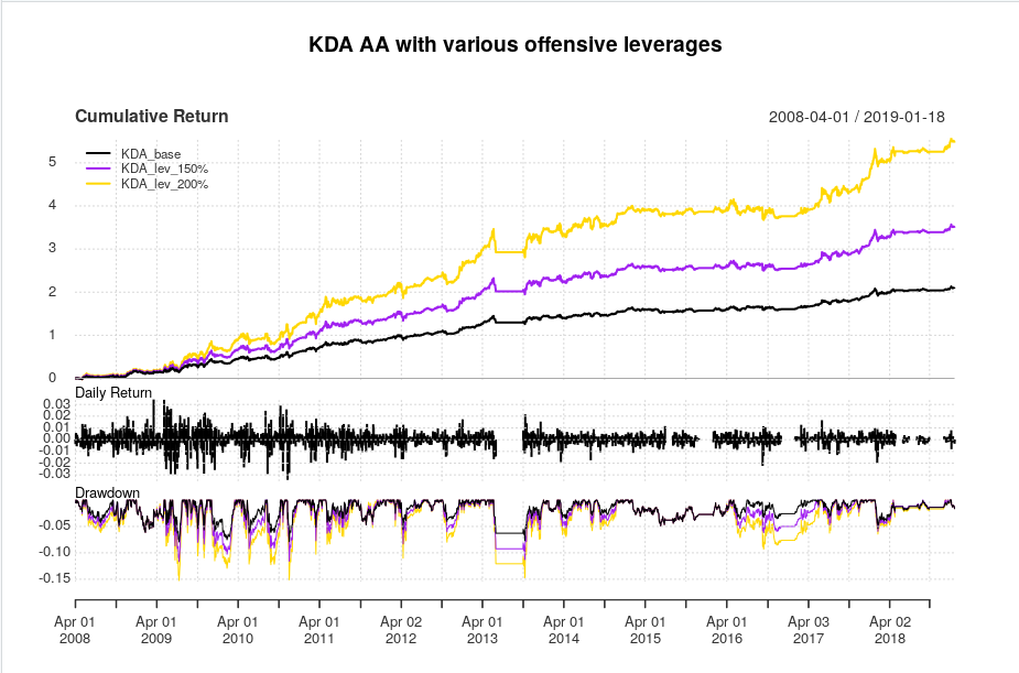
charts.PerformanceSummary(compare, colorset = c('black', 'purple', 'gold'),
main = "KDA AA with various offensive leverages")
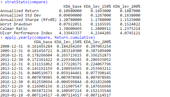
And here are the equity curves and statistics:
What appeals to me about this strategy, is that unlike most tactical asset allocation strategies, this strategy comes out relatively unscathed by the 2015-2016 whipsaws that hurt so many other tactical asset allocation strategies. However this strategy isn’t completely flawless, as sometimes, it decides that it’d be a great time to enter full risk-on mode and hit a drawdown, as evidenced by the drawdown curve. Nevertheless, the Calmar ratios are fairly solid for a tactical asset allocation rotation strategy, and even in a brutal 2018 that decimated all risk assets, this strategy managed to post a very noticeable *positive* return. On the downside, the leverage plan actually seems to *negatively* affect risk/reward characteristics in this strategy–that is, as leverage during aggressive allocations increases, characteristics such as the Sharpe and Calmar ratio actually *decrease*.
Overall, I think there are different aspects to unpack here–such as performances of risky assets as a function of the two canary universe assets, and a more optimal leverage plan. This was just the first attempt at combining two excellent ideas and seeing where the performance goes. I also hope that this strategy can have a longer backtest over at AllocateSmartly.
This post will review Kris Boudt’s datacamp course, along with introducing some concepts from it, discuss GARCH, present an application of it to volatility trading strategies, and a somewhat more general review of datacamp.
So, recently, Kris Boudt, one of the highest-ranking individuals pn the open-source R/Finance totem pole (contrary to popular belief, I am not the be-all end-all of coding R in finance…probably just one of the more visible individuals due to not needing to run a trading desk), taught a course on Datacamp on GARCH models.
Naturally, an opportunity to learn from one of the most intelligent individuals in the field in a hand-held course does not come along every day. In fact, on Datacamp, you can find courses from some of the most intelligent individuals in the R/Finance community, such as Joshua Ulrich, Ross Bennett (teaching PortfolioAnalytics, no less), David Matteson, and, well, just about everyone short of Doug Martin and Brian Peterson themselves. That said, most of those courses are rather introductory, but occasionally, you get a course that covers a production-tier library that allows one to do some non-trivial things, such as this course, which covers Alexios Ghalanos’s rugarch library.
Ultimately, the course is definitely good for showing the basics of rugarch. And, given how I blog and use tools, I wholly subscribe to the 80/20 philosophy–essentially that you can get pretty far using basic building blocks in creative ways, or just taking a particular punchline and applying it to some data, and throwing it into a trading strategy to see how it does.
But before we do that, let’s discuss what GARCH is.
While I’ll save the Greek notation for those that feel inclined to do a google search, here’s the acronym:
Auto-Regressive: past values are used as inputs to predict future values.
Conditional: the current value differs given a past value.
Heteroskedasticity: varying volatility. That is, consider the VIX. It isn’t one constant level, such as 20. It varies with respect to time.
Or, to summarize: “use past volatility to predict future volatility because it changes over time.”
Now, there are some things that we know from empirical observation about looking at volatility in financial time series–namely that volatility tends to cluster–high vol is followed by high vol, and vice versa. That is, you don’t just have one-off huge moves one day, then calm moves like nothing ever happened. Also, volatility tends to revert over longer periods of time. That is, VIX doesn’t stay elevated for protracted periods of time, so more often than not, betting on its abatement can make some money, (assuming the timing is correct.)
Now, in the case of finance, which birthed the original GARCH, 3 individuals (Glosten-Jagannathan-Runkle) extended the model to take into account the fact that volatility in an asset spikes in the face of negative returns. That is, when did the VIX reach its heights? In the biggest of bear markets in the financial crisis. So, there’s an asymmetry in the face of positive and negative returns. This is called the GJR-GARCH model.
Now, here’s where the utility of the rugarch package comes in–rather than needing to reprogram every piece of math, Alexios Ghalanos has undertaken that effort for the good of everyone else, and implemented a whole multitude of prepackaged GARCH models that allow the end user to simply pick the type of GARCH model that best fits the assumptions the end user thinks best apply to the data at hand.
So, here’s the how-to.
First off, we’re going to get data for SPY from Yahoo finance, then specify our GARCH model.
The GARCH model has three components–the mean model–that is, assumptions about the ARMA (basic ARMA time series nature of the returns, in this case I just assumed an AR(1)), a variance model–which is the part in which you specify the type of GARCH model, along with variance targeting (which essentially forces an assumption of some amount of mean reversion, and something which I had to use to actually get the GARCH model to converge in all cases), and lastly, the distribution model of the returns. In many models, there’s some in-built assumption of normality. In rugarch, however, you can relax that assumption by specifying something such as “std” — that is, the Student T Distribution, or in this case, “sstd”–Skewed Student T Distribution. And when one thinks about the S&P 500 returns, a skewed student T distribution seems most reasonable–positive returns usually arise as a large collection of small gains, but losses occur in large chunks, so we want a distribution that can capture this property if the need arises.
<pre class="wp-block-syntaxhighlighter-code brush: plain; notranslate">
require(rugarch)
require(quantmod)
require(TTR)
require(PerformanceAnalytics)

# get SPY data from Yahoo
getSymbols("SPY", from = '1990-01-01')

spyRets = na.omit(Return.calculate(Ad(SPY)))

# GJR garch with AR1 innovations under a skewed student T distribution for returns
gjrSpec = ugarchspec(mean.model = list(armaOrder = c(1,0)),
                      variance.model = list(model = "gjrGARCH",
                                            variance.targeting = TRUE),
                      distribution.model = "sstd")
</pre>
As you can see, with a single function call, the user can specify a very extensive model encapsulating assumptions about both the returns and the model which governs their variance. Once the model is specified,it’s equally simple to use it to create a rolling out-of-sample prediction–that is, just plug your data in, and after some burn-in period, you start to get predictions for a variety of metrics. Here’s the code to do that.
<pre class="wp-block-syntaxhighlighter-code brush: plain; notranslate">
# Use rolling window of 504 days, refitting the model every 22 trading days
t1 = Sys.time()
garchroll = ugarchroll(gjrSpec, data = spyRets,
n.start = 504, refit.window = "moving", refit.every = 22)
t2 = Sys.time()
print(t2-t1)

# convert predictions to data frame
garchroll = as.data.frame(garchroll)
</pre>
In this case, I use a rolling 504 day window that refits every 22 days(approximately 1 trading month). To note, if the window is too short,you may run into fail-to-converge instances, which would disallow converting the predictions to a data frame. The rolling predictions take about four minutes to run on the server instance I use, so refitting every single day is most likely not advised.
The
salient quantity here is the Sigma quantity–that is, the prediction
for daily volatility. This is the quantity that we want to compare
against the VIX.
So the strategy we’re going to be investigating is essentially what I’ve seen referred to as VRP–the Volatility Risk Premium in Tony Cooper’s seminal paper, Easy Volatility Investing.
The idea of the VRP is that we compare some measure of realized
volatility (EG running standard deviation, GARCH predictions from
past data) to the VIX, which is an implied volatility (so, purely
forward looking). The idea is that when realized volatility
(past/current measured) is greater than future volatility, people are
in a panic. Similarly, when implied volatility is greater than
realized volatility, things are as they should be, and it should be
feasible to harvest the volatility risk premium by shorting
volatility (analogous to selling insurance).
The instruments we’ll be using for this are ZIV and VXZ. ZIV
because SVXY is no longer supported on InteractiveBrokers or
RobinHood, and then VXZ is its long volatility counterpart.
We’ll be using close-to-close returns; that is, get the signal on Monday morning, and transact on Monday’s close, rather than observe data on Friday’s close, and transact around that time period as well(also known as magical thinking, according to Brian Peterson).
So, to comment on this strategy: this is definitely not something you will take and trade out of the box. Both variants of this strategy, when forced to choose a side, walk straight into the Feb 5 volatility explosion. Luckily, switching between ZIV and VXZ keeps the account from completely exploding in a spectacular failure. To note, both variants of the VRP strategy, GJR Garch and the 22 day rolling realized volatility, suffer their own period of spectacularly large drawdown–the historical volatility in 2007-2008, and currently, though this year has just been miserable for any reasonable volatility strategy, I myself am down 20%, and I’ve seen other strategists down that much as well in their primary strategies.
That said, I do think that over time, and if using the tail-end-of-the-curve instruments such as VXZ and ZIV (now that XIV is gone and SVXY no longer supported on several brokers such as Interactive Brokers and RobinHood), that there are a number of strategies that might be feasible to pass off as a sort of trading analogue to machine learning’s “weak learner”.
That said, I’m not sure how many vastly different types of ways to approach volatility trading there are that make logical sense from an intuitive perspective (that is, “these two quantities have this type of relationship, which should give a consistent edge in trading volatility” rather than “let’s over-optimize these two parameters until we eliminate every drawdown”).
While I’ve written about the VIX3M/VIX6M ratio in the past, which has formed the basis of my proprietary trading strategy, I’d certainly love to investigate other volatility trading ideas out in public. For instance, I’d love to start the volatility trading equivalent of an AllocateSmartly type website–just a compendium of a reasonable suite of volatility trading strategies, track them, charge a subscription fee, and let users customize their own type of strategies. However, the prerequisite for that is that there are a lot of reasonable ways to trade volatility that don’t just walk into tail-end events such as the 2007-2008 transition, Feb 5, and so on.
Furthermore, as some recruiters have told me that I should also cross-post my blog scripts on my Github, I’ll start doing that also, from now on.
*** One last topic: a general review of Datacamp. As some of you may know, I instruct a course on datacamp. But furthermore, I’ve spent quite a bit of time taking courses (particularly in Python) on there as well, thanks to having access by being an instructor.
Generally, here’s the gist of it: Datacamp is a terrific resource for getting your feet wet and getting a basic overview of what technologies are out there. Generally, courses follow a “few minutes of lecture, do exercises using the exact same syntax you saw in the lecture”, with a lot of the skeleton already written for you, so you don’t wind up endlessly guessing. Generally, my procedure will be: “try to complete the exercise, and if I fail, go back and look at the slides to find an analogous block of code, change some names, and fill in”.
Ultimately, if the world of data science, machine learning, and some quantitative finance is completely new to you–if you’re the kind of person that reads my blog, and completely glosses past the code: *this* is the resource for you, and I recommend it wholeheartedly. You’ll take some courses that give you a general tour of what data scientists, and occasionally, quants, do. And in some cases, you may have a professor in a fairly advanced field, like Kris Boudt, teach a fairly advanced topic, like the state-of-the art rugarch package (this *is* an industry-used package, and is actively maintained by Alexios Ghalanos, an economist at Amazon, so it’s far more than a pedagogical tool).
That said, for someone like me, who’s trying to port his career-capable R skills to Python to land a job (my last contract ended recently, so I am formally searching for a new role), Datacamp doesn’t *quite* do the trick–just yet. While there is a large catalog of courses, it does feel like there’s a lot of breadth, though not sure how much depth in terms of getting proficient enough to land interviews on the sole merits of DataCamp course completions. While there are Python course tracks (EG python developer, which I completed, and Python data analyst, which I also completed), I’m not sure they’re sufficient in terms of “this track was developed with partnership in industry–complete this capstone course, and we have industry partners willing to interview you”.
Also, from what I’ve seen of quantitative finance taught in Python, and having to rebuild all functions from numpy/pandas, I am puzzled as to how people do quantitative finance in Python without libraries like PerformanceAnalytics, rugarch, quantstrat, PortfolioAnalytics, and so on. Those libraries make expressing and analyzing investment ideas far more efficient, and removes a great chance of making something like an off-by-one error (also known as look-ahead bias in trading). So far, I haven’t seen the Python end of Datacamp dive deep into quantitative finance, and I hope that changes in the near future.
So, as a summary, I think this is a fantastic site for code-illiterate individuals to get their hands dirty and their feet wet with some coding, but I think the opportunity to create an economic, democratized, interest to career a-la-carte, self-paced experience is still very much there for the taking. And given the quality of instructors that Datacamp has worked with in the past (David Matteson–*the* regime change expert, I think–along with many other experts), I think Datacamp has a terrific opportunity to capitalize here.
So, if you’re the kind of person who glosses past the code: don’t gloss anymore. You can now take courses to gain an understanding of what my code does, and ask questions about it.
*** Thanks for reading.
NOTE: I am currently looking for networking opportunities and full-time roles related to my skill set. Feel free to download my resume or contact me on LinkedIn.
This post will investigate using Principal Components as part of a momentum strategy.
Recently, I ran across a post from David Varadi that I thought I’d further investigate and translate into code I can explicitly display (as David Varadi doesn’t). Of course, as David Varadi is a quantitative research director with whom I’ve done good work with in the past, I find that trying to investigate his ideas is worth the time spent.
So, here’s the basic idea: in an allegedly balanced universe, containing both aggressive (e.g. equity asset class ETFs) assets and defensive assets (e.g. fixed income asset class ETFs), that principal component analysis, a cornerstone in machine learning, should have some effectiveness at creating an effective portfolio.
I decided to put that idea to the test with the following algorithm:
Using the same assets that David Varadi does, I first use a rolling window (between 6-18 months) to create principal components. Making sure that the SPY half of the loadings is always positive (that is, if the loading for SPY is negative, multiply the first PC by -1, as that’s the PC we use), and then create two portfolios–one that’s comprised of the normalized positive weights of the first PC, and one that’s comprised of the negative half.
Next, every month, I use some momentum lookback period (1, 3, 6, 10, and 12 months), and invest in the portfolio that performed best over that period for the next month, and repeat.
require(PerformanceAnalytics)
require(quantmod)
require(stats)
require(xts)

symbols <- c("SPY", "EFA", "EEM", "DBC", "HYG", "GLD", "IEF", "TLT")

# get free data from yahoo
rets <- list()
getSymbols(symbols, src = 'yahoo', from = '1990-12-31')
for(i in 1:length(symbols)) {
  returns <- Return.calculate(Ad(get(symbols[i])))
  colnames(returns) <- symbols[i]
  rets[[i]] <- returns
}
rets <- na.omit(do.call(cbind, rets))

# 12 month PC rolling PC window, 3 month momentum window
pcPlusMinus <- function(rets, pcWindow = 12, momWindow = 3) {
  ep <- endpoints(rets)

  wtsPc1Plus <- NULL
  wtsPc1Minus <- NULL

  for(i in 1:(length(ep)-pcWindow)) {
    # get subset of returns
    returnSubset <- rets[(ep[i]+1):(ep[i+pcWindow])]

    # perform PCA, get first PC (I.E. pc1)
    pcs <- prcomp(returnSubset)
    firstPc <- pcs[[2]][,1]

    # make sure SPY always has a positive loading
    # otherwise, SPY and related assets may have negative loadings sometimes
    # positive loadings other times, and creates chaotic return series

    if(firstPc['SPY'] < 0) {
      firstPc <- firstPc * -1
    }

    # create vector for negative values of pc1
    wtsMinus <- firstPc * -1
    wtsMinus[wtsMinus < 0] <- 0
    wtsMinus <- wtsMinus/(sum(wtsMinus)+1e-16) # in case zero weights
    wtsMinus <- xts(t(wtsMinus), order.by=last(index(returnSubset)))
    wtsPc1Minus[[i]] <- wtsMinus

    # create weight vector for positive values of pc1
    wtsPlus <- firstPc
    wtsPlus[wtsPlus < 0] <- 0
    wtsPlus <- wtsPlus/(sum(wtsPlus)+1e-16)
    wtsPlus <- xts(t(wtsPlus), order.by=last(index(returnSubset)))
    wtsPc1Plus[[i]] <- wtsPlus
  }

  # combine positive and negative PC1 weights
  wtsPc1Minus <- do.call(rbind, wtsPc1Minus)
  wtsPc1Plus <- do.call(rbind, wtsPc1Plus)

  # get return of PC portfolios
  pc1MinusRets <- Return.portfolio(R = rets, weights = wtsPc1Minus)
  pc1PlusRets <- Return.portfolio(R = rets, weights = wtsPc1Plus)

  # combine them
  combine <-na.omit(cbind(pc1PlusRets, pc1MinusRets))
  colnames(combine) <- c("PCplus", "PCminus")

  momEp <- endpoints(combine)
  momWts <- NULL
  for(i in 1:(length(momEp)-momWindow)){
    momSubset <- combine[(momEp[i]+1):(momEp[i+momWindow])]
    momentums <- Return.cumulative(momSubset)
    momWts[[i]] <- xts(momentums==max(momentums), order.by=last(index(momSubset)))
  }
  momWts <- do.call(rbind, momWts)

  out <- Return.portfolio(R = combine, weights = momWts)
  colnames(out) <- paste("PCwin", pcWindow, "MomWin", momWindow, sep="_")
  return(list(out, wtsPc1Minus, wtsPc1Plus, combine))
}


pcWindows <- c(6, 9, 12, 15, 18)
momWindows <- c(1, 3, 6, 10, 12)

permutes <- expand.grid(pcWindows, momWindows)

stratStats <- function(rets) {
  stats <- rbind(table.AnnualizedReturns(rets), maxDrawdown(rets))
  stats[5,] <- stats[1,]/stats[4,]
  stats[6,] <- stats[1,]/UlcerIndex(rets)
  rownames(stats)[4] <- "Worst Drawdown"
  rownames(stats)[5] <- "Calmar Ratio"
  rownames(stats)[6] <- "Ulcer Performance Index"
  return(stats)
}

results <- NULL
for(i in 1:nrow(permutes)) {
  tmp <- pcPlusMinus(rets = rets, pcWindow = permutes$Var1[i], momWindow = permutes$Var2[i])
  results[[i]] <- tmp[[1]]
}
results <- do.call(cbind, results)
stats <- stratStats(results)
After a cursory look at the results, it seems the performance is fairly miserable with my implementation, even by the standards of tactical asset allocation models (the good ones have a Calmar and Sharpe Ratio above 1)
Here are histograms of the Calmar and Sharpe ratios.
These values are generally too low for my liking. Here’s a screenshot of the table of all 25 results.
While my strategy of choosing which portfolio to hold is different from David Varadi’s (momentum instead of whether or not the aggressive portfolio is above its 200-day moving average), there are numerous studies that show these two methods are closely related, yet the results feel starkly different (and worse) compared to his site.
I’d certainly be willing to entertain suggestions as to how to improve the process, which will hopefully create some more meaningful results. I also know that AllocateSmartly expressed interest in implementing something along these lines for their estimable library of TAA strategies, so I thought I’d try to do it and see what results I’d find, which in this case, aren’t too promising.
Thanks for reading.
NOTE: I am networking, and actively seeking a position related to my skill set in either Philadelphia, New York City, or remotely. If you know of a position which may benefit from my skill set, feel free to let me know. You can reach me on my LinkedIn profile here, or email me.
This post will discuss the idea of the geometric Calmar ratio — a way to modify the Calmar ratio to account for compounding returns.
So, one thing that recently had me sort of annoyed in terms of my interpretation of the Calmar ratio is this: essentially, the way I interpret it is that it’s a back of the envelope measure of how many years it takes you to recover from the worst loss. That is, if a strategy makes 10% a year (on average), and has a loss of 10%, well, intuition serves that from that point on, on average, it’ll take about a year to make up that loss–that is, a Calmar ratio of 1. Put another way, it means that on average, a strategy will make money at the end of 252 trading days.
But, that isn’t really the case in all circumstances. If an investment manager is looking to create a small, meager return for their clients, and is looking to make somewhere between 5-10%, then sure, the Calmar ratio approximation and interpretation makes sense in that context. Or, it makes sense in the context of “every year, we withdraw all profits and deposit to make up for any losses”. But in the context of a hedge fund trying to create large, market-beating returns for its investors, those hedge funds can have fairly substantial drawdowns.
In any case, in order to recover from such losses, it’s clear that a strategy would need to make back a lot more than what it lost. Lose 25%? 33% is the high water mark. Lose 33%? 50% to get back to even. Lose 50%? 100%. Beyond that? You get the idea.
In order to capture this dynamic, we should write a new Calmar ratio to express this idea.
So here’s a function to compute the geometric calmar ratio:
So, let's compare how some symbols stack up. We'll take a high-volatility name (AMZN), the good old S&P 500 (SPY), and a very low volatility instrument (SHY).
For my own proprietary volatility trading strategy, a strategy which has a Calmar above 2 (interpretation: finger in the air means that you make a new equity high every six months in the worst case scenario), here are the statistics:
> CalmarRatio(stratRetsAggressive[[2]]['2011::'])
                Close
Calmar Ratio 3.448497
> geomCalmar(stratRetsAggressive[[2]]['2011::'])
                     Close
Annualized Return 2.588094
Essentially, because of the nature of losses compounding, the geometric Calmar ratio will always be lower than the standard Calmar ratio, which is to be expected when dealing with the geometric nature of compounding returns.
Essentially, I hope that this gives individuals some thought about re-evaluating the Calmar Ratio.
Thanks for reading.
NOTES: registration for R/Finance 2018 is open. As usual, I’ll be giving a lightning talk, this time on volatility trading.
I am currently contracting and seek network opportunities, along with information about prospective full time roles starting in July. Those interested in my skill set can feel free to reach out to me on LinkedIn here.
This post will cover two aspects: the first will be a function to convert daily returns into a table of monthly returns, complete with drawdowns and annual returns. The second will be an interview I had with David Lincoln (now on youtube) to talk about the events of Feb. 5, 2018, and my philosophy on volatility trading.
So, to start off with, a function that I wrote that’s supposed to mimic PerforamnceAnalytics’s table.CalendarReturns is below. What table.CalendarReturns is supposed to do is to create a month X year table of monthly returns with months across and years down. However, it never seemed to give me the output I was expecting, so I went and wrote another function.
Here’s the code for the function:
require(data.table)
require(PerformanceAnalytics)
require(scales)
require(Quandl)

# helper functions
pastePerc <- function(x) {return(paste0(comma(x),"%"))}
rowGsub <- function(x) {x <- gsub("NA%", "NA", x);x}

calendarReturnTable <- function(rets, digits = 3, percent = FALSE) {

  # get maximum drawdown using daily returns
  dds <- apply.yearly(rets, maxDrawdown)

  # get monthly returns
  rets <- apply.monthly(rets, Return.cumulative)

  # convert to data frame with year, month, and monthly return value
  dfRets <- cbind(year(index(rets)), month(index(rets)), coredata(rets))

  # convert to data table and reshape into year x month table
  dfRets <- data.frame(dfRets)
  colnames(dfRets) <- c("Year", "Month", "Value")
  monthNames <- c("Jan", "Feb", "Mar", "Apr", "May", "Jun", "Jul", "Aug", "Sep", "Oct", "Nov", "Dec")
  for(i in 1:length(monthNames)) {
    dfRets$Month[dfRets$Month==i] <- monthNames[i]
  }
  dfRets <- data.table(dfRets)
  dfRets <- data.table::dcast(dfRets, Year~Month)

  # create row names and rearrange table in month order
  dfRets <- data.frame(dfRets)
  yearNames <- dfRets$Year
  rownames(dfRets) <- yearNames; dfRets$Year <- NULL
  dfRets <- dfRets[,monthNames]

  # append yearly returns and drawdowns
  yearlyRets <- apply.yearly(rets, Return.cumulative)
  dfRets$Annual <- yearlyRets
  dfRets$DD <- dds

  # convert to percentage
  if(percent) {
    dfRets <- dfRets * 100
  }

  # round for formatting
  dfRets <- apply(dfRets, 2, round, digits)

  # paste the percentage sign
  if(percent) {
    dfRets <- apply(dfRets, 2, pastePerc)
    dfRets <- apply(dfRets, 2, rowGsub)
    dfRets <- data.frame(dfRets)
    rownames(dfRets) <- yearNames
  }
  return(dfRets)
}
That covers it for the function. Now, onto volatility trading. Dodging the February short volatility meltdown has, in my opinion, been one of the best out-of-sample validators for my volatility trading research. My subscriber numbers confirm it, as I’ve received 12 new subscribers this month, as individuals interested in the volatility trading space have gained a newfound respect for the risk management that my system uses. After all, it’s the down months that vindicate system traders like myself that do not employ leverage in the up times. Those interested in following my trades can subscribe here. Furthermore, recently, I was able to get a chance to speak with David Lincoln about my background, and philosophy on trading in general, and trading volatility in particular. Those interested can view the interview here.
Thanks for reading.
NOTE: I am currently interested in networking, full-time positions related to my skill set, and long-term consulting projects. Those interested in discussing professional opportunities can find me on LinkedIn after writing a note expressing their interest.
This post will be about comparing a volatility signal using three different variations of implied volatility indices to predict when to enter a short volatility position.
In volatility trading, there are three separate implied volatility indices that have a somewhat long history for trading–the VIX (everyone knows this one), the VXV (more recently changed to be called the VIX3M), which is like the VIX, except for a three-month period), and the VXMT, which is the implied six-month volatility period.
This relationship gives investigation into three separate implied volatility ratios: VIX/VIX3M (aka VXV), VIX/VXMT, and VIX3M/VXMT, as predictors for entering a short (or long) volatility position.
One quick strategy to investigate is simple–the idea that the ratio should be below 1 (I.E. contango in implied volatility term structure) and decreasing (below a moving average). So when the ratio will be below 1 (that is, with longer-term implied volatility greater than shorter-term), and the ratio will be below its 60-day moving average, the strategy will take a position in XIV.
> stratStats(compare)
                              Short    Medium     Long
Annualized Return         0.5485000 0.6315000 0.638600
Annualized Std Dev        0.3874000 0.3799000 0.378900
Annualized Sharpe (Rf=0%) 1.4157000 1.6626000 1.685600
Worst Drawdown            0.5246983 0.5318472 0.335756
Calmar Ratio              1.0453627 1.1873711 1.901976
Ulcer Performance Index   3.7893478 4.6181788 5.244137
In other words, the VIX3M/VXMT sports the lowest drawdowns (by a large margin) with higher returns.
So, when people talk about which implied volatility ratio to use, I think this offers some strong evidence for the longer-out horizon as a predictor for which implied vol term structure to use. It’s also why it forms the basis of my subscription strategy.
Thanks for reading.
NOTE: I am currently seeking a full-time position (remote or in the northeast U.S.) related to my skill set demonstrated on this blog. Please message me on LinkedIn if you know of any opportunities which may benefit from my skill set.