A Python Investigation of a New Proposed Short Vol ETF–SVIX

This post will be about analyzing SVIX–a proposed new short vol ETF that aims to offer the same short vol exposure as XIV used to–without the downside of, well, blowing up in 20 minutes due to positive feedback loops. As I’m currently enrolled in a Python bootcamp, this was one of my capstone projects on A/B testing, so, all code will be in Python (again).

So, first off, with those not familiar, there was an article about this proposed ETF published about a month ago. You can read it here. The long story short is that this ETF is created by one Stuart Barton, who also manages InvestInVol. From conversations with Stuart, I can vouch for the fact that he strikes me as very knowledgeable in the vol space, and, if I recall correctly, was one of the individuals that worked on the original VXX ETF at Barclay’s. So when it comes to creating a newer, safer vehicle for trading short-term short vol, I’d venture to think he’s about as good as any.

In any case, here’s a link to my Python notebook, ahead of time, which I will now discuss here, on this post.

So first off, we’ll start by getting the data, and in case anyone forgot what XIV did in 2018, here’s a couple of plots.

import numpy as np
import pandas as pd
import scipy.stats as stats
import matplotlib.pyplot as plt
from pandas_datareader import data
import datetime as dt
from datetime import datetime

# get XIV from a public dropbox -- XIV had a termination event Feb. 5 2018, so this is archived data.

xiv = pd.read_csv("https://dl.dropboxusercontent.com/s/jk6der1s5lxtcfy/XIVlong.TXT", parse_dates=True, index_col=0)

# get SVXY data from Yahoo finance
svxy = data.DataReader('SVXY', 'yahoo', '2016-01-01')
#yahoo_xiv = data.DataReader('XIV', 'yahoo', '1990-01-01')

# yahoo no longer carries XIV because the instrument blew up, need to find it from historical sources
xiv_returns = xiv['Close'].pct_change()
svxy_returns = svxy['Close'].pct_change()

xiv['Close'].plot(figsize=(20,10))
plt.show()
xiv['2016':'2018']['Close'].plot(figsize=(20,10))

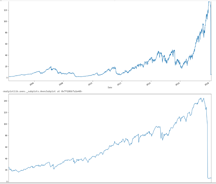
Yes, for those new to the blog, that event actually happened, and in the span of 20 minutes (my trading system got to the sideline about a week before, and even had I been in–which I wasn’t–I would have been in ZIV), during which time XIV blew up in after-hours trading. Immediately following, SVXY (which survived), deleveraged to a 50% exposure.

In any case, here’s the code to get SVIX data from my dropbox, essentially to the end of 2019, after I manually did some work on it because the CBOE has it in a messy format, and then to combine it with the combined XIV + SVXY returns data. (For the record, the SVIX hypothetical performance can be found here on the CBOE website)

# get formatted SVIX data from my dropbox (CBOE has it in a mess)

svix = pd.read_csv("https://www.dropbox.com/s/u8qiz7rh3rl7klw/SHORTVOL_Data.csv?raw=1", header = 0, parse_dates = True, index_col = 0)
svix.columns = ["Open", "High", "Low", "Close"]
svix_rets = svix['Close'].pct_change()

# put data set together

xiv_svxy = pd.concat([xiv_returns[:'2018-02-07'],svxy_returns['2018-02-08':]], axis = 0)
xiv_svxy_svix = pd.concat([xiv_svxy, svix_rets], axis = 1).dropna()
xiv_svxy_svix.tail()

final_data = xiv_svxy_svix
final_data.columns = ["XIV_SVXY", "SVIX"]

One thing that can be done right off the bat (which is a formality) is check if the distributions of XIV+SVXY or SVIX are normal in nature.

print(stats.describe(final_data['XIV_SVXY']))
print(stats.describe(final_data['SVIX']))
print(stats.describe(np.random.normal(size=10000)))

Which gives the following output:

DescribeResult(nobs=3527, minmax=(-0.9257575757575758, 0.1635036496350366), mean=0.0011627123490346562, variance=0.0015918321320673623, skewness=-4.325358554250933, kurtosis=85.06927230848028)
DescribeResult(nobs=3527, minmax=(-0.3011955533480766, 0.16095949898733686), mean=0.0015948970447533636, variance=0.0015014216189676208, skewness=-1.0811171524703087, kurtosis=4.453114992142524)
DescribeResult(nobs=10000, minmax=(-4.024990382591559, 4.017237262611489), mean=-0.012317646021121993, variance=0.9959681097965573, skewness=0.00367629631713188, kurtosis=0.0702696931810931)

Essentially, both of them are very non-normal (obviously), so any sort of statistical comparison using t-tests isn’t really valid. That basically leaves the Kruskal-Wallis test and Wilcoxon signed rank test to see if two data sets are different. From a conceptual level, the idea is fairly straightforward: the Kruskal-Wallis test is analogous to a two-sample independent t-test to see if one group differs from another, while the Wilcoxon signed rank test is analogous to a t-test of differences, except both use ranks of the observations rather than the actual values themselves.

Here’s the code for that:

stats.kruskal(final_data['SVIX'], final_data['XIV_SVXY'])
stats.wilcoxon(final_data['SVIX'], final_data['XIV_SVXY'])

With the output:

KruskalResult(statistic=0.8613306385456933, pvalue=0.3533665896055551)
WilcoxonResult(statistic=2947901.0, pvalue=0.0070668195307847575)

Essentially, when seen as two completely independent instruments, there isn’t enough statistical evidence to reject the idea that SVIX has no difference in terms of the ranks of its returns compared to XIV + SVXY, which would make a lot of sense, considering that for both, Feb. 5, 2018 was their worst day, and there wasn’t much of a difference between the two instruments prior to Feb. 5. In contrast, when considering the two instruments from the perspective of SVIX becoming the trading vehicle for what XIV used to be, and then comparing the differences against a 50% leveraged SVXY, then SVIX is the better instrument with differences that are statistically significant at the 1% level.

Basically, SVIX accomplishes its purpose of being an improved take on XIV/SVXY, because it was designed to be just that, with statistical evidence of exactly this.

One other interesting question to ask is when exactly did the differences in the Wilcoxon signed rank test start appearing? After all, SVIX is designed to have been identical to XIV prior to the crash and SVXY’s deleveraging. For this, we can use the endpoints function for Python I wrote in the last post.

# endpoints function

def endpoints(df, on = "M", offset = 0):
    """
    Returns index of endpoints of a time series analogous to R's endpoints
    function. 
    Takes in: 
        df -- a dataframe/series with a date index
         
        on -- a string specifying frequency of endpoints
         
        (E.G. "M" for months, "Q" for quarters, and so on)
         
        offset -- to offset by a specified index on the original data
        (E.G. if the data is daily resolution, offset of 1 offsets by a day)
        This is to allow for timing luck analysis. Thank Corey Hoffstein.
    """
     
    # to allow for familiarity with R
    # "months" becomes "M" for resampling
    if len(on) > 3:
        on = on[0].capitalize()
     
    # get index dates of formal endpoints
    ep_dates = pd.Series(df.index, index = df.index).resample(on).max()
     
    # get the integer indices of dates that are the endpoints
    date_idx = np.where(df.index.isin(ep_dates))
     
    # append zero and last day to match R's endpoints function
    # remember, Python is indexed at 0, not 1
    date_idx = np.insert(date_idx, 0, 0)
    date_idx = np.append(date_idx, df.shape[0]-1)
    if offset != 0:
        date_idx = date_idx + offset
        date_idx[date_idx < 0] = 0
        date_idx[date_idx > df.shape[0]-1] = df.shape[0]-1
    out = np.unique(date_idx)
    return out   

ep = endpoints(final_data)

dates = []
pvals = []
for i in range(0, (len(ep)-12)):
  data_subset = final_data.iloc[(ep[i]+1):ep[i+12]]
  pval = stats.wilcoxon(data_subset['SVIX'], data_subset['XIV_SVXY'])[1]
  date = data_subset.index[-1]
  dates.append(date)
  pvals.append(pval)
wilcoxTS = pd.Series(pvals, index = dates)
wilcoxTS.plot(figsize=(20,10))

wilcoxTS.tail(30)

The last 30 points in this monthly time series looks like this:

2017-11-29    0.951521
2017-12-28    0.890546
2018-01-30    0.721118
2018-02-27    0.561795
2018-03-28    0.464851
2018-04-27    0.900470
2018-05-30    0.595646
2018-06-28    0.405771
2018-07-30    0.228674
2018-08-30    0.132506
2018-09-27    0.085125
2018-10-30    0.249457
2018-11-29    0.230020
2018-12-28    0.522734
2019-01-30    0.224727
2019-02-27    0.055854
2019-03-28    0.034665
2019-04-29    0.019178
2019-05-30    0.065563
2019-06-27    0.071348
2019-07-30    0.056757
2019-08-29    0.129120
2019-09-27    0.148046
2019-10-30    0.014340
2019-11-27    0.006139
2019-12-26    0.000558
dtype: float64

And the corresponding chart looks like this:

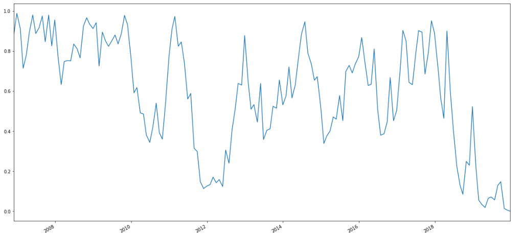
Essentially, about six months after Feb. 5, 2018–I.E. about six months after SVXY deleveraged, we see the p-value for yearly rolling Wilcoxon signed rank tests (measured monthly) plummet and stay there.

So, the long story short is: once SVIX starts to trade, it should be the way to place short-vol, near-curve bets, as opposed to the 50% leveraged SVXY that traders must avail themselves with currently (or short VXX, with all of the mechanical and transaction risks present in that regard).

That said, from having tested SVIX with my own volatility trading strategy (which those interested can subscribe to, though in fair disclosure, this should be a strategy that diversifies a portfolio, and it’s a trend follower that was backtested in a world without Orange Twitler creating price jumps every month), the performance improves from backtesting with the 50% leveraged SVXY, but as I *dodged* Feb. 5, 2018, the results are better, but the risk is amplified as well, because there wasn’t really a protracted sideways market the likes of which we’ve seen the past couple of years for a long while.

In any case, thanks for reading.

NOTE: I am currently seeking a full-time opportunity either in the NYC or Philadelphia area (or remotely). Feel free to reach out to me on my LinkedIn, or find my resume here.